import regression
import matplotlib.pyplot as plt
import matplotlib.ticker as mtick
import numpy as np
if __name__ == "__main__":
srcX, y = regression.loadDataSet('data/lwr.txt');
m,n = srcX.shape
srcX = np.concatenate((srcX[:, 0], np.power(srcX[:, 0],2)), axis=1)
X = regression.standardize(srcX.copy())
X = np.concatenate((np.ones((m,1)), X), axis=1)
rate = 0.1
maxLoop = 1000
epsilon = 0.01
predicateX = regression.standardize(np.matrix([[8, 64]]))
predicateX = np.concatenate((np.ones((1,1)), predicateX), axis=1)
result, t = regression.lwr(rate, maxLoop, epsilon, X, y, predicateX, 1)
theta, errors, thetas = result
result2, t = regression.lwr(rate, maxLoop, epsilon, X, y, predicateX, 0.1)
theta2, errors2, thetas2 = result2
fittingFig = plt.figure()
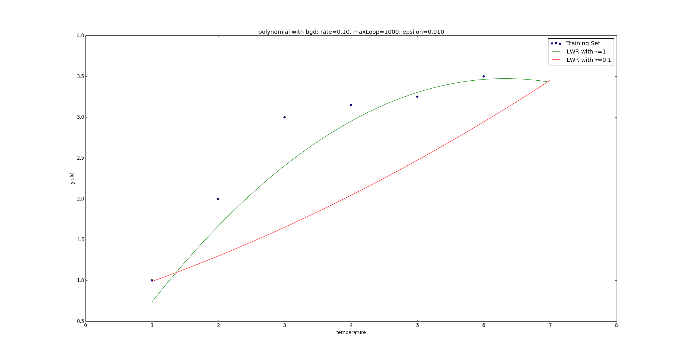
title = 'polynomial with bgd: rate=%.2f, maxLoop=%d, epsilon=%.3f'%(rate,maxLoop,epsilon)
ax = fittingFig.add_subplot(111, title=title)
trainingSet = ax.scatter(srcX[:, 0].flatten().A[0], y[:,0].flatten().A[0])
print theta
print theta2
xx = np.linspace(1, 7, 50)
xx2 = np.power(xx,2)
yHat1 = []
yHat2 = []
for i in range(50):
normalizedSize = (xx[i]-xx.mean())/xx.std(0)
normalizedSize2 = (xx2[i]-xx2.mean())/xx2.std(0)
x = np.matrix([[1,normalizedSize, normalizedSize2]])
yHat1.append(regression.h(theta, x.T))
yHat2.append(regression.h(theta2, x.T))
fittingLine1, = ax.plot(xx, yHat1, color='g')
fittingLine2, = ax.plot(xx, yHat2, color='r')
ax.set_xlabel('temperature')
ax.set_ylabel('yield')
plt.legend([trainingSet, fittingLine1, fittingLine2], ['Training Set', r'LWR with $\tau$=1', r'LWR with $\tau$=0.1'])
plt.show()
errorsFig = plt.figure()
ax = errorsFig.add_subplot(111)
ax.yaxis.set_major_formatter(mtick.FormatStrFormatter('%.2e'))
ax.plot(range(len(errors)), errors)
ax.set_xlabel('Number of iterations')
ax.set_ylabel('Cost J')
plt.show()
|

 wechat
 alipay