"""
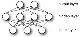
This tutorial introduces the multilayer perceptron using Theano.
A multilayer perceptron is a logistic regressor where
instead of feeding the input to the logistic regression you insert a
intermediate layer, called the hidden layer, that has a nonlinear
activation function (usually tanh or sigmoid) . One can use many such
hidden layers making the architecture deep. The tutorial will also tackle
the problem of MNIST digit classification.
.. math::
f(x) = G( b^{(2)} + W^{(2)}( s( b^{(1)} + W^{(1)} x))),
References:
- textbooks: "Pattern Recognition and Machine Learning" -
Christopher M. Bishop, section 5
"""
from __future__ import print_function
__docformat__ = 'restructedtext en'
import os
import sys
import timeit
import numpy
import theano
import theano.tensor as T
from logistic_sgd import LogisticRegression, load_data
class HiddenLayer(object):
    def __init__(self, rng, input, n_in, n_out, W=None, b=None,
                 activation=T.tanh):
        """
        Typical hidden layer of a MLP: units are fully-connected and have
        sigmoidal activation function. Weight matrix W is of shape (n_in,n_out)
        and the bias vector b is of shape (n_out,).

        NOTE : The nonlinearity used here is tanh

        Hidden unit activation is given by: tanh(dot(input,W) + b)

        :type rng: numpy.random.RandomState
        :param rng: a random number generator used to initialize weights

        :type input: theano.tensor.dmatrix
        :param input: a symbolic tensor of shape (n_examples, n_in)

        :type n_in: int
        :param n_in: dimensionality of input

        :type n_out: int
        :param n_out: number of hidden units

        :type activation: theano.Op or function
        :param activation: Non linearity to be applied in the hidden
                           layer
        """
        self.input = input
if W is None:
W_values = numpy.asarray(
rng.uniform(
low=-numpy.sqrt(6. / (n_in + n_out)),
high=numpy.sqrt(6. / (n_in + n_out)),
size=(n_in, n_out)
),
dtype=theano.config.floatX
)
if activation == theano.tensor.nnet.sigmoid:
W_values *= 4
W = theano.shared(value=W_values, name='W', borrow=True)
if b is None:
b_values = numpy.zeros((n_out,), dtype=theano.config.floatX)
b = theano.shared(value=b_values, name='b', borrow=True)
self.W = W
self.b = b
lin_output = T.dot(input, self.W) + self.b
self.output = (
lin_output if activation is None
else activation(lin_output)
)
self.params = [self.W, self.b]
class MLP(object):
"""Multi-Layer Perceptron Class
A multilayer perceptron is a feedforward artificial neural network model
that has one layer or more of hidden units and nonlinear activations.
Intermediate layers usually have as activation function tanh or the
sigmoid function (defined here by a ``HiddenLayer`` class) while the
top layer is a softmax layer (defined here by a ``LogisticRegression``
class).
"""
def __init__(self, rng, input, n_in, n_hidden, n_out):
"""Initialize the parameters for the multilayer perceptron
:type rng: numpy.random.RandomState
:param rng: a random number generator used to initialize weights
:type input: theano.tensor.TensorType
:param input: symbolic variable that describes the input of the
architecture (one minibatch)
:type n_in: int
:param n_in: number of input units, the dimension of the space in
which the datapoints lie
:type n_hidden: int
:param n_hidden: number of hidden units
:type n_out: int
:param n_out: number of output units, the dimension of the space in
which the labels lie
"""
self.hiddenLayer = HiddenLayer(
rng=rng,
input=input,
n_in=n_in,
n_out=n_hidden,
activation=T.tanh
)
self.logRegressionLayer = LogisticRegression(
input=self.hiddenLayer.output,
n_in=n_hidden,
n_out=n_out
)
self.L1 = (
abs(self.hiddenLayer.W).sum()
+ abs(self.logRegressionLayer.W).sum()
)
self.L2_sqr = (
(self.hiddenLayer.W ** 2).sum()
+ (self.logRegressionLayer.W ** 2).sum()
)
self.negative_log_likelihood = (
self.logRegressionLayer.negative_log_likelihood
)
self.errors = self.logRegressionLayer.errors
self.params = self.hiddenLayer.params + self.logRegressionLayer.params
self.input = input
def test_mlp(learning_rate=0.01, L1_reg=0.00, L2_reg=0.0001, n_epochs=1000,
dataset='mnist.pkl.gz', batch_size=20, n_hidden=500):
"""
Demonstrate stochastic gradient descent optimization for a multilayer
perceptron
This is demonstrated on MNIST.
:type learning_rate: float
:param learning_rate: learning rate used (factor for the stochastic
gradient
:type L1_reg: float
:param L1_reg: L1-norm's weight when added to the cost (see
regularization)
:type L2_reg: float
:param L2_reg: L2-norm's weight when added to the cost (see
regularization)
:type n_epochs: int
:param n_epochs: maximal number of epochs to run the optimizer
:type dataset: string
:param dataset: the path of the MNIST dataset file from
http://www.iro.umontreal.ca/~lisa/deep/data/mnist/mnist.pkl.gz
"""
datasets = load_data(dataset)
train_set_x, train_set_y = datasets[0]
valid_set_x, valid_set_y = datasets[1]
test_set_x, test_set_y = datasets[2]
n_train_batches = train_set_x.get_value(borrow=True).shape[0] // batch_size
n_valid_batches = valid_set_x.get_value(borrow=True).shape[0] // batch_size
n_test_batches = test_set_x.get_value(borrow=True).shape[0] // batch_size
print('... building the model')
index = T.lscalar()
x = T.matrix('x')
y = T.ivector('y')
rng = numpy.random.RandomState(1234)
classifier = MLP(
rng=rng,
input=x,
n_in=28 * 28,
n_hidden=n_hidden,
n_out=10
)
cost = (
classifier.negative_log_likelihood(y)
+ L1_reg * classifier.L1
+ L2_reg * classifier.L2_sqr
)
test_model = theano.function(
inputs=[index],
outputs=classifier.errors(y),
givens={
x: test_set_x[index * batch_size:(index + 1) * batch_size],
y: test_set_y[index * batch_size:(index + 1) * batch_size]
}
)
validate_model = theano.function(
inputs=[index],
outputs=classifier.errors(y),
givens={
x: valid_set_x[index * batch_size:(index + 1) * batch_size],
y: valid_set_y[index * batch_size:(index + 1) * batch_size]
}
)
gparams = [T.grad(cost, param) for param in classifier.params]
updates = [
(param, param - learning_rate * gparam)
for param, gparam in zip(classifier.params, gparams)
]
train_model = theano.function(
inputs=[index],
outputs=cost,
updates=updates,
givens={
x: train_set_x[index * batch_size: (index + 1) * batch_size],
y: train_set_y[index * batch_size: (index + 1) * batch_size]
}
)
print('... training')
patience = 10000
patience_increase = 2
improvement_threshold = 0.995
validation_frequency = min(n_train_batches, patience // 2)
best_validation_loss = numpy.inf
best_iter = 0
test_score = 0.
start_time = timeit.default_timer()
epoch = 0
done_looping = False
while (epoch < n_epochs) and (not done_looping):
epoch = epoch + 1
for minibatch_index in range(n_train_batches):
minibatch_avg_cost = train_model(minibatch_index)
iter = (epoch - 1) * n_train_batches + minibatch_index
if (iter + 1) % validation_frequency == 0:
validation_losses = [validate_model(i) for i
in range(n_valid_batches)]
this_validation_loss = numpy.mean(validation_losses)
print(
'epoch %i, minibatch %i/%i, validation error %f %%' %
(
epoch,
minibatch_index + 1,
n_train_batches,
this_validation_loss * 100.
)
)
if this_validation_loss < best_validation_loss:
if (
this_validation_loss < best_validation_loss *
improvement_threshold
):
patience = max(patience, iter * patience_increase)
best_validation_loss = this_validation_loss
best_iter = iter
test_losses = [test_model(i) for i
in range(n_test_batches)]
test_score = numpy.mean(test_losses)
print((' epoch %i, minibatch %i/%i, test error of '
'best model %f %%') %
(epoch, minibatch_index + 1, n_train_batches,
test_score * 100.))
if patience <= iter:
done_looping = True
break
end_time = timeit.default_timer()
print(('Optimization complete. Best validation score of %f %% '
'obtained at iteration %i, with test performance %f %%') %
(best_validation_loss * 100., best_iter + 1, test_score * 100.))
print(('The code for file ' +
os.path.split(__file__)[1] +
' ran for %.2fm' % ((end_time - start_time) / 60.)), file=sys.stderr)
if __name__ == '__main__':
test_mlp()
|

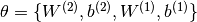
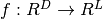 ,其中D是输入向量x的大小,L是输出向量f(x)的大小,矩阵表现为:
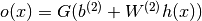
 , b是偏差向量,W是权重矩阵,G和s是激活函数。
 构成隐藏层。
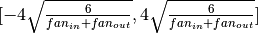
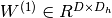 是连接输入向量和隐藏层的权重矩阵。Wi代表输入单元到第i个隐藏单元的权重。一般选择tanh作为s的激活函数,使用
 或者使用逻辑sigmoid函数,
 。
。 。
。 。
。 可以使用反向传播算法获得(连续微分的特殊形式),Theano可以自动计算这一微分过程。
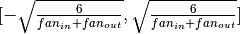
 wechat
 alipay