import os
import tensorflow as tf
W = tf.Variable(tf.zeros([5, 1]), name="weights")
b = tf.Variable(0., name="bias")
def read_csv(batch_size, file_name, record_defaults):
filename_queue = tf.train.string_input_producer(
[os.path.dirname(__file__) + "/" + file_name])
reader = tf.TextLineReader(skip_header_lines=1)
key, value = reader.read(filename_queue)
decoded = tf.decode_csv(value, record_defaults=record_defaults)
return tf.train.shuffle_batch(decoded,
batch_size=batch_size,
capacity=batch_size * 50,
min_after_dequeue=batch_size)
def inference(X):
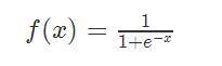
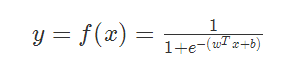
return tf.sigmoid(tf.matmul(X, W) + b)
def loss(X, Y):
return tf.reduce_mean(tf.nn.sigmoid_cross_entropy_with_logits(
tf.matmul(X, W) + b, Y))
def inputs():
passenger_id, survived, pclass, name, sex, age, sibsp, parch, ticket, fare,\
cabin, embarked = read_csv(100,
"train.csv",
[[0.0], [0.0], [0], [""],
[""], [0.0], [0.0], [0.0],
[""], [0.0], [""], [""]])
is_first_class = tf.to_float(tf.equal(pclass, [1]))
is_second_class = tf.to_float(tf.equal(pclass, [2]))
is_third_class = tf.to_float(tf.equal(pclass, [3]))
gender = tf.to_float(tf.equal(sex, ["female"]))
features = tf.transpose(
tf.pack([is_first_class,
is_second_class,
is_third_class,
gender,
age]))
survived = tf.reshape(survived, [100, 1])
return features, survived
def train(total_loss):
learning_rate = 0.01
return tf.train.GradientDescentOptimizer(learning_rate).minimize(
total_loss)
def evaluate(sess, X, Y):
predicted = tf.cast(inference(X) > 0.5, tf.float32)
print sess.run(tf.reduce_mean(tf.cast(tf.equal(predicted, Y), tf.float32)))
with tf.Session() as sess:
tf.initialize_all_variables().run()
X, Y = inputs()
total_loss = loss(X, Y)
train_op = train(total_loss)
coord = tf.train.Coordinator()
threads = tf.train.start_queue_runners(sess=sess, coord=coord)
training_steps = 1000
for step in range(training_steps):
sess.run([train_op])
if step % 100 == 0:
print "loss at step ", step, ":", sess.run([total_loss])
evaluate(sess, X, Y)
coord.request_stop()
coord.join(threads)
|

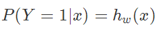 ,似然函数为
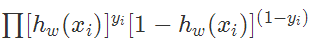 ,那么对数似然函数为
 ,
,
 而这个正则化项一般会采用L1范数或者L2范数。其形式分别为:
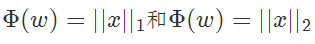
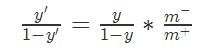 其中,$m-$为反例数目,$m+$为正例数目)
 wechat
 alipay